Research – Maxwell Fishelson

Conference Publications

From External to Swap Regret 2.0: An Efficient Reduction for Large Action Spaces
Yuval Dagan, Constantinos Daskalakis, Maxwell Fishelson, Noah Golowich
STOC 2024 [paper][long-talk][slides]

Online Learning and Solving Infinite Games with an ERM Oracle
Angelos Assos, Idan Attias, Yuval Dagan, Constantinos Daskalakis, Maxwell Fishelson
COLT 2023 [paper][short-talk][long-talk][slides]

Near-Optimal No-Regret Learning for Correlated Equilibria in Multi-Player General-Sum Games
Ioannis Anagnostides, Constantinos Daskalakis, Gabriele Farina, Maxwell Fishelson, Noah Golowich, Tuomas Sandholm
STOC 2022 [paper][short-talk][long-talk]

Near-Optimal No-Regret Learning in General Games
Constantinos Daskalakis, Maxwell Fishelson, Noah Golowich
NeurIPS 2021 Oral Presentation [paper]

Multi-item Non-truthful Auctions Achieve Good Revenue
Constantinos Daskalakis, Maxwell Fishelson, Brendan Lucier, Vasilis Syrgkanis and Santhoshini Velusamy
EC 2020 [paper] [talk] [low-level talk]

Journal Publications

Multi-item Non-truthful Auctions Achieve Good Revenue
Constantinos Daskalakis, Maxwell Fishelson, Brendan Lucier, Vasilis Syrgkanis and Santhoshini Velusamy
SICOMP 2022 [paper] [journal]

Pattern Avoidance Over a Hypergraph
Maxwell Fishelson, Benjamin Gunby
Electronic Journal of Combinatorics 2021 [paper] [journal]

Resume

From External to Swap Regret 2.0: An Efficient Reduction for Large Action Spaces

In the setting of online learning, the benefits of “No-Swap-Regret” learning are many. As opposed to the classic “No-External-Regret” learning, in the game setting, a No-Swap-Regret learner is robust to an adversary that has knowledge of their learning algorithm. Moreover, No-Swap-Regret learning is sufficient for many important online learning metrics, such as calibration. Most importantly of all, in multi-player or general-sum games, when all players use No-Swap-Regret learning for repeated decision making, their time-averaged strategies converge to a “correlated equilibrium” of the game. This is in contrast with No-External-Regret learning, which only guarantees time-averaged convergence to “coarse correlated equilibrium”. In a world where computing a Nash equilibrium is PPAD-hard, correlated equilibrium is the gold standard of computationally feasible equilibria. It’s often hard to argue that a coarse correlated equilibrium is even a point of stability.

How is it, then, that practical applications of No-External-Regret learning far outreach those of No-Swap-Regret learning? Perhaps the main reason is the dependence of No-Swap-Regret guarantees on the number of actions. No-External-Regret algorithms, such as MWU, achieve an average external regret of $\epsilon$ after $T=O\left(\frac{\log N}{\epsilon^2}\right)$ rounds of learning, where $N$ represents the number of actions available to the learner. On the other hand, classic No-Swap-Regret algorithms [BM07, SL05] require poly-$N$ many iterations: achieving $\epsilon$ swap regret after $T=O\left(\frac{N \log N}{\epsilon^2}\right)$ rounds of learning. In many practical applications, this dependence on $N$ is limiting when the set of actions available to the learner is massive. For example, a learner could be tasked with tuning the parameters of a neural net.

This begs the question: is there a way to perform No-Swap-Regret learning with an improved, even poly-logarithmic, dependence on $N$? In this work, we answer this question in the affirmative! Our algorithm TreeSwap achieves an average swap regret of $\epsilon$ after $T=(\log N)^{\tilde{O}(1/\epsilon)}$ rounds. Moreover, in the styles of Blum Mansour and Stoltz Lugosi, our algorithm is a black-box reduction from external regret learning. Accordingly, if the adversary selects losses from a class of bounded Littlestone dimension $L$ (the standard notion of dimensionality for external regret learning), our algorithm guarantees $\epsilon$ swap regret for $T= L^{\tilde{O}(1/\epsilon ) }$. This means achieving No-Swap-Regret is possible even with $N$ infinite, as long as $L$ is finite.

The drawback of achieving poly-logarithmic dependence on $N$ is an exponential dependence on $1/\epsilon$. We establish a lower bound of $ T = \Omega(1) \cdot \min \left\{ \exp(O(\epsilon^{-1/6})),\frac{N}{\log^{12} (N)\cdot \epsilon^2} \right\} $, showing that this exponential dependence on $1/\epsilon$ is inevitable for any swap regret algorithm with poly-logarithmic dependence on $N$. Put another way, we construct an adversary who forces any learner to incur a total swap regret of $\frac{T}{\text{polylog}(T)}$. The adversary does so using only $N=4T$ actions, and only selecting rewards satisfying $\|u\|_1 \leq 1$: a class of constant Littlestone Dimension.

Both the upper and lower bounds come from tree-based constructions. But where are these trees coming from? Here, I hope to offer some of the intuition behind the constructions, and elucidate a hidden connection to the classic Blum Mansour algorithm.

Inspired by the 2005 work of Stoltz and Lugosi, in 2007 Blum and Mansour devised an algorithm (BM) that achieves a swap regret of $O\left(\sqrt{NT\log(N)}\right)$. It’s an algorithm that takes an arbitrary No-External-Regret algorithm, and uses it as a black-box. The $O\left(\sqrt{NT\log(N)}\right)$ swap regret comes from plugging Multiplicative Weight Updates (MWU) into the black box. However, if we’re dealing with a large set of actions $N \geq T$, this guarantee is merely $O(T)$ and is therefore meaningless. The question is: can BM achieve sub-linear swap regret when $N \geq T$ for an appropriately-chosen black box No-External-Regret algorithm? The answer is yes.

The BM algorithm runs as follows. For each action $i \in [N]$, we create an instance of our black-box No-External-Regret algorithm $\text{Alg}_i$. At every time step $t$, each instance $\text{Alg}_i$ suggests a mixed action $q_i^{(t)} \in \Delta(N)$. These form the rows of an $N \times N$ Markov-chain matrix $Q^{(t)}$. The algorithm then computes the stationary distribution of this matrix $x^{(t)} \in \Delta(N)$ and uses that as its final output for the round. When it receives feedback from the adversary $\ell^{(t)} \in [0,1]^N$, BM updates each instance $\text{Alg}_i$ with feedback $x^{(t)}[i]\ell^{(t)}$: the loss scaled by the weight given to action $i$.

The guarantee of BM is that the swap regret of the whole algorithm is equal to the sum of the external regrets of the black box instances. The problem is that, if the instances have even constant regret, summing over all $N$ instances, we will have linear swap regret for $N \geq T$. So on the surface, it seems that any selection of black-box algorithm cannot guarantee sub-linear swap regret. The secret is to take advantage of how our selection of black-box algorithm can affect the resulting Markov chains of BM. The goal is to select an algorithm such that, no matter what the adversary does, only a small number $S < T$ of actions ever have non-zero weight in the stationary distributions of the resulting Markov chains. If we can guarantee this, then we guarantee that only $S$ instances incur non-zero loss over all $T$ rounds of learning, and only $S$ instances have non-zero regret.

How could we do such a thing? For simplicity in this moment, let’s assume, at each time step, each black-box instance $\text{Alg}_i$ suggests a pure action $j$. The ensuing “Markov chain” for this time step is a directed graph where every vertex has one outgoing edge (1-out digraph). A graph with $N$ vertices and $N$ edges (assuming it’s connected in an undirected sense) contains one cycle, and a bunch of trees rooted in nodes of that cycle. A “stationary distribution” of this Markov chain is the uniform distribution over the nodes of this cycle. Our goal is to have only $S$ distinct nodes ever appear in the cycle over all $T$ rounds of learning. The critical question becomes: is there a No-External-Regret algorithm that can be used as a black-box which ensures only a small set of nodes ever appear in the cycle, regardless of what the adversary does? The answer is yes, and the secret is to use a No-External-Regret algorithm that has small support!

As a warm-up, we consider a “lazy” version of Follow The Leader (FTL). Like classic FTL, the algorithm recommends the action with minimal cumulative loss. However, lazy FTL doesn’t update every round. It repeatedly plays an action for an epoch of rounds. Only at the end of an epoch does it update, computing the best historical action at that time and playing that action repeatedly for the next epoch.

We will plug this algorithm into BM, instantiating black-box instances for each action $i \in N$ in a clever way, using varying epoch lengths. We will do so in such a way that the resulting BM Markov chains have a certain structure over the time steps of learning. Namely, we hope to ensure that the stationary distribution cycles progress as follows.

For $M,d$ integers satisfying $T=M^d$, we consider a subset $\mathcal{S}$ of the $N$ nodes that form an $M$-ary, depth-$d$ tree. That is, a collection of $\sum_{i=0}^d M^i$ nodes, and if $N$ is smaller than this, we can allow for repeats as we will see in a bit. Over all the time steps of learning, we will ensure that only nodes in $\mathcal{S}$ ever belong to the Markov chain cycles. This is achieved as follows. The tree has $T$ leaves that we enumerate $\ell_0,\cdots,\ell_{T-1}$. For each $t \in [0,T-1]$, we will ensure that our 1-out digraph Markov chain will contain the path from the root to the leaf $\ell_t$, as well as an edge from $\ell_t$ back to the root. We don’t need to specify the other edges of the Markov chain, as the presence of this cycle alone will ensure that the uniform distribution over the nodes on the root-to-$\ell_t$ path will constitute a stationary distribution. Importantly, when the stationary distribution is not unique (e.g. there are multiple cycles), BM only requires that any stationary distribution be played. So, we need not be concerned about the other edges. We could imagine, for example, that all the nodes outside of $\mathcal{S}$ point to the root of the tree at all the time steps.

In many ways, this would seem to give us what we want, but in other ways, it seems impossible.

Firstly, indeed the recommendations of the black-box instances, which correspond to the outgoing edges of the nodes, occur in epochs like lazy-FTL. For a time step $t$, letting $\sigma_1\sigma_2\cdots\sigma_d$ denote the base-$M$ representation of $t$, we will have the directed edge from the root to its child of index $\sigma_1$; that child will have an edge to its child of index $\sigma_2$, etc. So, for example, the root has an outgoing edge to its zeroth child for the first $T/M$ rounds. Then, it points at its first child for rounds $t \in [T/M + 1,2T/M]$; then its third child for rounds $t \in [2T/M + 1,3T/M]$ etc.

But hold on just a moment! Our plan was to ensure that the Markov chains progress in this fashion regardless of what actions the adversary takes. How could such a precarious structure arise in the face of an adaptive adversary?! Surely the adversary can feed loss into BM such that the black-box No-External-Regret algorithm for the root doesn’t recommend each of its children in sequential epochs!

Here’s the idea. We will ensure that the stationary distributions take this form by not specifying in advance which actions map to which nodes in the tree. In an online fashion, we determine the actions corresponding to the different tree nodes and even what actions belong to $\mathcal{S}$ in the first place! This is simply done by observing what the algorithms recommend as a result of the adversary.

We can tie-break in such a way that all $N$ of our Lazy-FTL instances initially recommend the same action $A$ before incurring any loss. This action will represent the root of the tree, and we will initialize its lazy-FTL instance with an epoch length of $T/M$, matching the epoch length of the outgoing edges of the root. At time $t=T/M$, this root instance $\text{Alg}_A$ updates and suggests some action $B$. This will “reveal” that action $B$ is what is represented by the node that is the first (second, but we zero indexed) child of the root. We can accordingly instantiate $\text{Alg}_B$ with epoch length $T/M^2$, matching the epoch length of the outgoing edges of nodes at depth $1$ of the tree. If $B$ did not appear earlier in the tree, we can get away with only specifying the epoch length now, as the algorithm has received no loss and just suggested $A$ up until this point.

Even in the event that $\text{Alg}_B$ had been instantiated earlier in the tree with a different epoch length, it’s okay to have multiple black-box instances for this single action. We can hallucinate a duplicate action $B’$ that is equivalent to $B$ and instantiate $\text{Alg}_{B’}$ with the desired epoch length. This only strengthens our No-Swap-Regret guarantee. Typically, we only compete with hindsight transformations of our actions that map ALL of the weight placed on some action $B$ to a fixed action. With two black-box instances for action $B$, a No-Swap-Regret guarantee means our loss competes with the larger set of hindsight transformations, wherein the historical weight placed on action $B$ is partitioned into the weight placed on $B$ and $B’$, and each of these parts can be mapped to different fixed actions. Forcing both parts to map to the same fixed action, as is the case in swap regret, only weakens the benchmark.

Also, we previously said that we hoped that our BM algorithm would have small support $S < T$. However here, $|\mathcal{S}| = T(1+1/M+1/M^2+\cdots+1/M^d)$. Thankfully though, we can split into two cases. The total support coming from internal nodes of the algorithm is $T(1/M+1/M^2+\cdots+1/M^d) \leq \frac{T}{M-1}$. Now indeed there are $T$ black-box instances corresponding to the leaves that each incur some non-zero regret. However, because we, at each time step, play a stationary distribution that is uniform over a root-to-leaf path of length $d+1$, only a $\frac{1}{d+1}$ fraction of the loss is distributed to the leaf algorithms, and the total swap regret contribution coming from these actions is $\leq \frac{T}{d+1}$. Tuning parameters $M = \log T$ and $d = \log T / \log \log T$, we have $T = M^d$ and both $\frac{T}{M-1}$ and $\frac{T}{d+1}$ sub-linear, albeit logarithmically so.

Woo! We found a black-box algorithm that makes BM have sub-linear support (ignoring the set of leaf actions that have a sub-linear total swap regret). Have we achieved sub-linear swap regret in total? Not quite. In order to do all this reasoning, we wanted our black-box algorithm to have pure action output, which we achieved by forgoing regularization. But you can’t just forgo regularization! That’s what makes No-External-Regret learning possible. When summing the external regrets of these unregularized algorithms at the end, we will still get stuck with linear swap regret.

Here’s the KICKER. The whole tree analysis had nothing to do with $N$. The structure of $\mathcal{S}$ was purely in terms of $T$, and we just “threw away” or “never gave any loss” to the extra actions. So, we could have had way more than $N$ actions total, and still have used this construction that has non-leaf support $\leq \frac{T}{\text{polylog}(T)}$. So, what if we “run” BM, not with a black-box instance for each action in $N$, but one for each of the infinitely many points on the simplex $\Delta (N)$! What if, rather than using lazy-FTL as our black-box algorithm, we use lazy-MWU, defined similarly with epochs of repeated actions, but now the repeated actions are mixed ones. Importantly, these “mixed action outputs” of MWU are “pure actions” on the simplex. The “root” of the tree is simply the uniform distribution, as that is what is suggested by MWU prior to any incurred loss. Everything about the previous construction holds, and using the classic analysis of Blum Mansour, we have

$$\begin{aligned} &\text{Swap Regret(Lazy-MWU BM)}\\ &= \sum_{\text{internal node actions }i} \text{Regret}(\text{Alg}_i) + \sum_{\text{leaf node actions }i} \text{Regret}(\text{Alg}_i) + \sum_{\text{other actions }i} \text{Regret}(\text{Alg}_i)\\ &\leq \sqrt{T\cdot|\text{internal nodes in }\mathcal{S}|\cdot \log(N)}+\frac{T}{d+1}+0\\&= \frac{T \log(N)}{\sqrt{M-1}}+\frac{T}{d+1}\\&=\frac{T\log(N)}{\text{polylog}(T)} \end{aligned}$$

as desired. Moreover, and not mentioned explicitly in the paper, because we are effectively running BM with a black-box algorithm for every point on the simplex, our algorithm actually achieves the $\frac{T \log(N)}{\text{polylog}(T)}$ swap regret guarantee FOR ALL swap functions $\Delta (N) \to \Delta (N)$, not just the linear maps $\Delta (N) \to \Delta (N)$ covered by distributional swap regret.

I call this “bananas swap regret”, though it’s not formally defined as low-distributional-swap-regret is the sufficient performance measure to achieve the guarantees described earlier. But, if you’re also a potassium-enjoyer, this is perhaps something to keep in mind.

The lower bound tree construction is also inspired by Blum Mansour. If an adversary is to force all learners to incur $\Omega\left(\frac{T}{\text{polylog}(T)}\right)$ swap regret, she must at the very least force a BM learner to do so. And, the only way to achieve that is to force the stationary distribution to progress according to a DFS tree traversal as is done here!

Concurrent work of Binghui and Aviad

Online Learning and Solving Infinite Games with an ERM Oracle

Accepted to the 36th Annual Conference on Learning Theory (COLT 2023), this work demonstrates that the online learning of a hypothesis class $H$ is possible, even when $H$ is infinite, as long as $H$ has finite Littlestone Dimension and we have ERM oracle access to $H$. An Empirical Risk Minimization (ERM) oracle will simply take some historical observations and find the hypothesis in $H$ that has minimal loss on these observations. In every structured setting of online learning where we have successful algorithms, we also have the ability to compute ERM. In this sense, it is a reasonable oracle model to consider. In contrast, all of the past work on the online learning of infinite hypothesis classes with finite Littlestone dimension relies on the Standard Optimal Algorithm (SOA) oracle model. SOA involves partitioning the set of feasible hypotheses several times, and computing the Littlestone dimension of each partition. In contrast with ERM, computation of SOA isn’t efficient even for finite learning settings. For a finite hypothesis class of size $n$, in polynomial time, we cannot even distinguish between the class having constant Littlestone dimension and the maximal $O(\log n)$. If we hope to obtain the optimal rates (in terms of Littlestone dimension) for online learning, we must make the SOA oracle assumption. The question of this paper is, under a more reasonable oracle model, though we will not obtain optimal rates, can we online learn at any reasonable rate under a feasible oracle model? The answer is yes.

The other contribution of this work is to study learning in infinite games under the ERM oracle model. Not only do we obtain positive results in this setting, but the algorithms suggested by the oracle model happen to be the “double-oracle” algorithms that are the most successful at solving large games in practice, like blotto and MARL. On the other hand, the algorithms suggested by the SOA oracle model don’t seem to have any practical use. The fact that the algorithms arising from the theoretical oracle model of ERM parallel those most effective in the real world only further emphasizes the importance of the model.

Near-Optimal No-Regret Learning for Correlated Equilibria in Multi-Player General-Sum Games

Accepted to the 54th ACM Symposium on Theory of Computing (STOC 2022), this work demonstrates that Blum-Mansour OMWU and Stoltz-Lugosi OMWU achieve poly-logarithmic swap and internal regret respectively in the game setting. These are the classic algorithms for achieving more sophisticated notions of regret by using a no-external regret algorithm as a black box. This work builds on the ideas of Chen and Peng who, in 2020, established an $O(T^{1/4})$ swap-regret bound for Blum-Mansour OMWU as well as the poly-logarithmic external-regret techniques established by Costis Daskalakis, Noah Golowich, and myself.

I was honored with the opportunity to present this work at STOC 2022, which was hosted in Rome this year! I was super excited because it was my first ever in-person conference. Up to this point, every single conference I had attended was made virtual due to the pandemic, dating back to the start of my research career in the summer of 2020. So, I had to go all out. Here’s the talk:

Near-Optimal No-Regret Learning in General Games

Overview

Awarded an Oral Presentation at the thirty-fifth conference on Neural Information Processing Systems (NeurIPS 21), this work establishes that Optimistic Hedge – a common variant of multiplicative-weights-updates with recency bias – attains $poly(\log T)$ regret in multi-player general-sum games. In particular, when every player of a game uses Optimistic Hedge to iteratively update her strategy in response to the history of play, then after $T$ rounds of interaction, each player experiences total regret that is $poly(\log T)$. This proof was a huge milestone in the space of multi-agent learning theory, attaining an exponential improvement on the previous best-known $O(T^{1/4})$ regret attainable in general-sum games.

Background

Modern machine learning applications are often tasked with learning in dynamic and potentially adversarial environments. This is in strict contrast with the foundational assumptions of classical machine learning. The traditional setting involves a single learner investigating a static environment, such as a fixed data set of traffic images. However, as machine learning becomes an increasingly ubiquitous tool in the modern world, these learning environments are rarely static. They are composed of several different learning agents all trying to optimize decision making, such as several companies in a shared economy trying to learn optimal pricing. In these settings, how one learner chooses to learn will impact the environment and impact how the others are learning. In this sense, a choice of a learning algorithm is analogous to a choice of a strategy in a game. These settings have led to a recent explosion of research on game theory interfaced with statistical learning.

The studying of online learning from an adversarial perspective was popularized back in 2006 with the work of Cesa-Bianchi and Lugosi. This work discussed the Follow-The-Regularized-Leader (FTRL) algorithm and demonstrated that a learner making decisions according to FTRL in a repeated, adversarial environment will only experience a “regret” of $O(\sqrt{T} )$ over $T$ time-step iterations of learning. Regret is a notion of loss incurred by the learner over this process. It is a comparison between the amount of loss they actually incurred versus the amount of loss they would have incurred had they chosen the best fixed action in hindsight: a meaningful benchmark. It was a break-through work when it came out, as it began to address the problem of learning in these dynamic environments which better model the modern world. It also came with a matching lower bound, that no algorithm could achieve regret better than $O(\sqrt{T})$ in the purely adversarial setting.

However, a main open question remained: is a purely adversarial model too pessimistic? Under a more realistic model, can we improve on $O(\sqrt{T})$? Rather than assuming the feedback we receive from the world is the absolute worst-case scenario, what if we assume that it is the product of the actions of other learning agents? Indeed, even in the setting where the environment is composed of learning agents playing a purely-adversarial zero-sum game, there is some guaranteed regularity that comes from the fact that all agents involved are using some robust algorithm for learning.

In 2015, Syrgkanis et. al. made the first major breakthrough in this direction [SALS15]. Awarded the Best Paper Award at NeurIPS 2015, this work demonstrated that all players in a game running a modified algorithm “Optimistic FTRL” for decision making will experience regret at most $O(T^{1/4})$. This was the first result to crack the $O(\sqrt{T})$ barrier, and it got the whole world of theoretical machine learning investigating if it was possible to further improve this bound.

This investigation was only concluded 6 years later through this work of Constantinos Daskalakis, Noah Golowich, and myself. We demonstrated that Optimistic Hedge, a common variant of Optimistic FTRL, attains $poly(\log(T))$ regret in multi-player general-sum games. This was an exponential improvement on the previously-best-known regret bound. For this discovery, we were awarded an Oral Presentation (top 50 papers out of 9000 submissions) at the NeurIPS 2021 conference.

Math

The crucial thing that separates the multi-agent game-theoretic setting of online learning from the adversarial setting is a guarantee that we refer to as “high-order smoothness”. What this means is that, if we look at the sequence of loss vectors experienced by each of the players over time, we can upper-bound the magnitude of the first, second, third, … $h^{\text{th}}$-order finite derivatives of the sequence. In the adversarial setting, the loss vector could be shifting wildly with the intention of throwing off the Optimistic Hedge algorithm. In the game setting though, even if the game is purely adversarial (zero-sum), there is some regularity guarantee that stems from the fact that all players are using the same Optimistic Hedge algorithm to govern their strategic dynamics. If all players except one are playing sequences of strategies that are smooth over time (having bounded high-order derivative), it will lead to a loss vector that is smooth over time for that one player as her experienced loss is a function of the strategies of others. In turn, since the mixed strategy she plays according to Optimistic Hedge is a function of the cumulative loss, her strategy vectors will be guaranteed smooth over time. This leads to an inductive argument that demonstrates that all players have high-order smooth strategies and losses.

Along the way of this inductive argument, there are some neat combinatorial lemmas that come into play but aren’t in the spotlight of our write-up. I’m using this blog post to give some of these arguments a little exposition!

Lemma B.5: The Magic of Softmax

The weight that Optimistic Hedge places on strategy $j$ at time step $t$ is \[\phi_j\left(-\eta \cdot \bar{\ell}^{(t)}_1, -\eta \cdot \bar{\ell}^{(t)}_2, \cdots -\eta \cdot \bar{\ell}^{(t)}_n\right)\] where $\bar{\ell}^{(t)}_i = \sum_{\tau = 1}^{t-1} \ell^{(\tau)}_i + \ell^{(t-1)}_i$ is the cumulative loss incurred for action $i$ (with some recency bias) and \[\phi_j(z_1,\cdots,z_n) = \frac{\exp(z_j)}{\sum_{i=1}^n \exp(z_i)}\] is the softmax function. A crucial step to this inductive argument is a bound on the Taylor coefficients of softmax. We want to show the following

\[
\frac{1}{k!}\sum_{t \in [n]^k} \left|\frac{\partial^k \phi_j(0)}{\partial z_{t_1} \partial z_{t_2}\cdots \partial z_{t_k}}\right| \leq \frac{1}{n}e^{\frac{k+1}{2}}
\]

Namely, we can think of the quantity we are trying to bound as the following: choose a $t_1$ from $1$ to $n$; take the derivative $\frac{\partial \phi_j}{\partial z_{t_1}}$; choose another $t_2$ from $1$ to $n$; take the derivative $\frac{\partial^2 \phi_j}{\partial z_{t_1}\partial z_{t_2}}$; repeat this process $k$ times until we have $\frac{\partial^k \phi_j}{\partial z_{t_1} \partial z_{t_2}\cdots \partial z_{t_k}}$. The quantity of interest comes from summing over all the possible choices of $(t_1,\cdots,t_k) \in [n]^k$ of the magnitude of $\frac{\partial^k \phi_j}{\partial z_{t_1} \partial z_{t_2}\cdots \partial z_{t_k}}$ evaluated at $0$.

Now, everybody learning about neural nets for the first time learns about the wonders of the sigmoid function as a non-linear activation $\sigma(x) = \frac{e^x}{e^x+1}$. The main reason for this is it has such a beautiful derivative, making it ideal for back propagation: $\sigma'(x)=\sigma(x)(1-\sigma(x))$. Softmax is the multidimensional extension of sigmoid and accordingly has a similarly nice derivative. This will form the basis of the argument. We have
\[\frac{\partial \phi_j}{\partial z_j} = \phi_j(1-\phi_j) \qquad \qquad \frac{\partial \phi_j}{\partial z_i} = -\phi_j\phi_i\]

These $(1-\phi_j)$ terms are gonna appear all throughout the analysis. We abbreviate them $\phi^*_j = 1 – \phi_j$ and call them “perturbed $\phi$s”. We notice something interesting: when we take the derivative of a $\phi$ or a perturbed $\phi$ relative to any $z_i$, we are left with the product of two $\phi$s (perhaps perturbed, perhaps not)
\[\frac{\partial \phi_j}{\partial z_j} = \phi_j\phi^*_j \qquad \frac{\partial \phi_j}{\partial z_i} = -\phi_j\phi_i \qquad \frac{\partial \phi^*_j}{\partial z_j} = -\phi_j\phi^*_j \qquad \frac{\partial \phi^*_j}{\partial z_i} = \phi_j\phi_i \]

This is going to have interesting implications on the value of $\frac{\partial^k \phi_j}{\partial z_{t_1} \partial z_{t_2}\cdots \partial z_{t_k}}$. Let $\phi^{?}$ denote a $\phi$ that may or may not be perturbed. We see the following.

Before taking any derivatives, we have a single term: $\phi_j$
After one derivative, we have a product of the form: $\pm \phi^?_j\phi^?_{t_1}$
After two derivatives, we have: $\pm \phi^?_j\phi^?_{t_1}\phi^?_{t_2} \pm \phi^?_j\phi^?_{t_1}\phi^?_{t_2}$
After three derivatives, we have: $\pm\phi^?_j\phi^?_{t_1}\phi^?_{t_2}\phi^?_{t_3}\pm\phi^?_j\phi^?_{t_1}\phi^?_{t_2}\phi^?_{t_3}\pm\phi^?_j\phi^?_{t_1}\phi^?_{t_2}\phi^?_{t_3}\pm\phi^?_j\phi^?_{t_1}\phi^?_{t_2}\phi^?_{t_3}\pm\phi^?_j\phi^?_{t_1}\phi^?_{t_2}\phi^?_{t_3}\pm\phi^?_j\phi^?_{t_1}\phi^?_{t_2}\phi^?_{t_3}$
After $k$ derivatives, we have the sum of $k!$ terms each consisting of $(k+1)$ $\phi$s

This comes from the product rule of differentiation. If we have a product of $\phi$s and take the derivative with respect to some $z_i$, we get
\begin{align*}
\frac{\partial}{\partial z_i} \phi^?_a \phi^?_b \phi^?_c &= \left ( \frac{\partial}{\partial z_i} \phi^?_a \right ) \phi^?_b \phi^?_c+\phi^?_a \left ( \frac{\partial}{\partial z_i} \phi^?_b \right ) \phi^?_c+\phi^?_a\phi^?_b \left ( \frac{\partial}{\partial z_i} \phi^?_c \right )\\
&= (\phi^?_a\phi^?_i)\phi^?_b\phi^?_c+\phi^?_a(\phi^?_b\phi^?_i)\phi^?_c+\phi^?_a\phi^?_b(\phi^?_c\phi^?_i)
\end{align*}

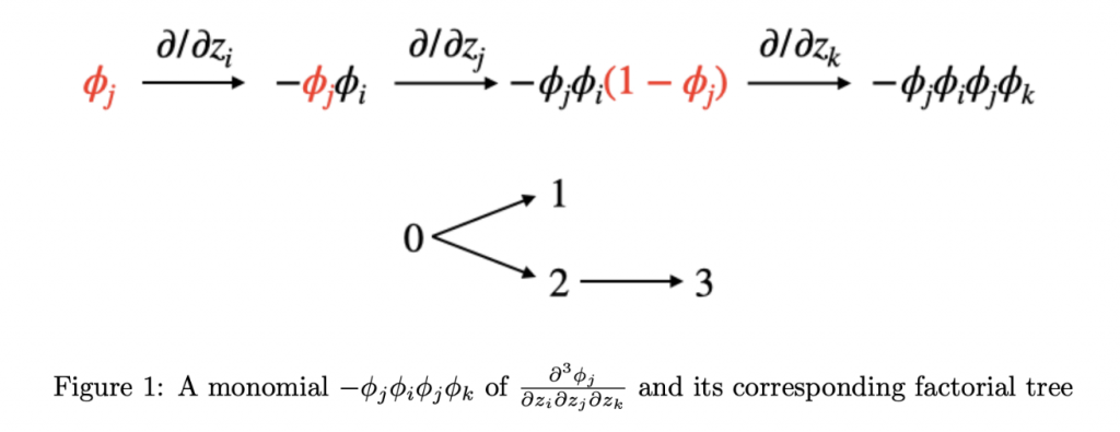
That is, for each $\phi$ in the product, we have a corresponding term in the resulting summation that comes from taking the derivative of that $\phi$. So, at the end of the process of evaluating $\frac{\partial^k \phi_j}{\partial z_{t_1} \partial z_{t_2}\cdots \partial z_{t_k}}$, we are left with a sum of $k!$ terms. We can enumerate these terms via the following generative process. At each time step $i$ from $1$ to $k$, we will transform a product of $i$ $\phi$s into a product of $(i+1)$ $\phi$s by selecting one of the $i$ $\phi$s and taking the derivative of that $\phi$ with respect to $z_{t_i}$. Going into the first derivative, we initialize our product to just be $\phi_j$. This is a product of a singular $\phi$, and we have 1 choice of $\phi$ to select for differentiation. Taking the derivative leaves us with a product of two $\phi$s. So, at the second derivative, we have 2 choices of $\phi$ for differentiation, each choice leaving us with a product of 3 $\phi$s. This goes on until we have a product of $k$ $\phi$s and $k$ choices of $\phi$ to select for the final derivative. In this way, we can think of a bijection between the $k!$ terms in the final summation and combinatorial structures we refer to as “factorial trees”.

Define a factorial tree to be a directed graph on vertices $0,1,\cdots,k$. Each vertex $i$ except $0$ has exactly one incoming edge from some vertex $j < i$. There are $k!$ such trees: one choice for the parent of $1$, two choices for the parent of $2$, etc. The factorial tree corresponding to a particular term will have, for all $i$, the parent of $i$ be the index of the $\phi$ that was selected for differentiation when taking the $i^{\text{th}}$ derivative in the generative process (using $0$ indexing).

The quantity of interest is the absolute value of the sum over all factorial trees of the corresponding product evaluated at $0$. We upper bound this by the sum of the absolute values of the products, which will enable us to just ignore the $\pm$ signs throughout the generative process.
\[\left|\sum_{\text{factorial trees }f} \pm \phi^?_{j}(0) \phi^?_{t_1}(0) \phi^?_{t_2}(0)\cdots \phi^?_{t_k}(0)\right| \leq \sum_{\text{factorial trees }f} \phi^?_{j}(0) \phi^?_{t_1}(0) \phi^?_{t_2}(0)\cdots \phi^?_{t_k}(0)\]

What each product will evaluate to when you plug in $0$ is entirely dependent on how many of the $\phi$s are perturbed. We see
\[\phi_j(0)=\frac{1}{n} \qquad \phi_j^*(0)=1-\frac{1}{n}\]

Therefore, we can bound $\phi^?_{j} \phi^?_{t_1} \phi^?_{t_2}\cdots \phi^?_{t_k} \leq (1/n)^{\text{number of unperturbed 𝜙s in the product}}$. Let’s formally go through our generative process to determine which $\phi$s are perturbed. To review
\[\left | \frac{\partial \phi_j}{\partial z_j}\right | = \phi_j\phi^*_j \qquad \left | \frac{\partial \phi_j}{\partial z_i}\right | = \phi_j\phi_i \qquad \left | \frac{\partial \phi^*_j}{\partial z_j}\right | = \phi_j\phi^*_j \qquad \left | \frac{\partial \phi^*_j}{\partial z_i}\right | = \phi_j\phi_i \]

We can interpret these differentiation rules as follows:

Say we are taking the derivative with respect to $z_i$ of a $\phi_j$. If $i \ne j$, then we will add an unperturbed $\phi_i$ to the end of the current product. However, if $i=j$, then we will add a perturbed $\phi^*_i$ to the end of the product.
If the $\phi$ that is chosen for differentiation is perturbed: $\phi^*_j$, it becomes unperturbed: $\phi_j$

These rules are a complete description of the behavior of these derivatives. Note, for example, that we can interpret $\left | \frac{\partial \phi^*_j}{\partial z_j} \right | = \phi_j\phi^*_j$ as the unperturbation of an existing term $\phi^*_j \to \phi_j$ as well as the addition of a new perturbed term $\phi^*_j$ since the derivative with respect to $z_j$ was directed at a $\phi^*_j$ with matching index $j$.

This leads to a clean parallel in the setting of factorial trees. We label the vertices of the factorial trees $0,1,2,\cdots,k$ with the corresponding indeces of derivation $j,t_1,t_2,\cdots,t_k$. Then, we can say the following. A vertex $i$ corresponds to a perturbed $\phi^*_{t_i}$ in the final product if and only if the parent of $i$ had the same label $t_i$ and if vertex $i$ has no children. That is, the term $\phi^*_{t_i}$ was perturbed when it got added, and it never got unperturbed as it was never selected for differentiation. We call such a leaf that has the same label as its parent a “petal”.

Wow, that was a lot of set up. But are you ready for the…

*•.BEAUTIFUL COMBINATORICS.•*

So, we have boiled the desired quantity down to the following. We are summing over all possible labelings $t \in [n]^k$. For each such labeling, we sum over all possible factorial trees the quantity $(1/n)^{\text{number of non-petal vertices}}=(1/n)^{k+1}\cdot n^{\text{number of petals}}$. The beautiful double count: rather than fixing the labeling and summing over all possible trees, let’s fix the tree and sum over all possible labelings! Letting $P_{f,t}$ denote the number of petals on tree $f$ with labeling $t$, we have
\begin{align*}
\frac{1}{k!} \sum_{t \in [n]^k}\sum_{\text{factorial trees }f} (1/n)^{k+1-P_{f,t}} &= \frac{1}{k!} \sum_{\text{factorial trees }f} \left((1/n)^{k+1} \sum_{t \in [n]^k}n^{P_{f,t}}\right)\\
&= \frac{1}{n}\mathbb{E}_f \left[ \mathbb{E}_t \left[n^{P_{f,t}}\right ]\right]
\end{align*}

For a fixed tree $f$, the random variable $P_{f,t}$ in $t$ has a very simple interpretation. $f$ has some fixed set of leaves $L_f$. For a random labeling $t \sim \mathcal{U}\left([n]^k\right)$, each leaf $\ell \in L_f$ will have the same label as its parent with probability $1/n$, independent of all other leaves. Therefore,
\[\mathbb{E}_t \left[n^{P_{f,t}}\right ] = \prod_{\ell \in L_f}\left(\frac{1}{n}\cdot n + \frac{n-1}{n} \cdot 1\right) \leq 2^{|L_f|}\]

We finish by bounding $\frac{1}{n}\mathbb{E}_f \left[2^{|L_f|}\right]$. For a specific vertex $\ell \in [0,k]$, we note that $\ell \in L_f$ if and only if it is not the parent of any vertex $\ell+1,\cdots,k$. So,
\begin{equation}
\Pr_{f}[\ell \in L_f] = \prod_{i=\ell+1}^{k} \frac{i-1}{i} = \frac{\ell}{k}
\end{equation}

Now, unlike the previous argument involving labels, these leaf events are not independent. Fortunately though, the correlation is negative here and works in our favor for an upper bound. That is, conditioning on one vertex $\ell$ being a leaf, it is even less likely that other vertices are leaves, as the vertices $\ell+1,\cdots,k$ have one fewer alternative option for their parent. We are able to show via an inductive argument that for any vertex set $S \subseteq [0,k]$
\begin{equation}
\Pr_{f}[S \subseteq L_f] \leq \prod_{\ell \in S} \frac{\ell}{k}
\end{equation}

This establishes a coupling between $L_f$ and a random subset $R \subseteq [0,k]$ generated from $k+1$ mutually independent coin flips, where we include $\ell \in R$ with probability $\frac{\ell}{k}$ for all $\ell \in [0,k]$. Therefore,
\begin{align*}
\frac{1}{n}\mathbb{E}_f \left[2^{|L_f|}\right] &\leq \frac{1}{n}\prod_{\ell=0}^k \left(\frac{\ell}{k}\cdot 2 + \frac{k-\ell}{k} \cdot 1\right)\\
&= \frac{1}{n}\prod_{\ell=0}^k \left(1+\frac{\ell}{k}\right)\\
&\leq \frac{1}{n}\exp\left(\sum_{\ell=0}^k \frac{\ell}{k}\right)\\
&=\frac{1}{n}e^{\frac{k+1}{2}}
\end{align*}
as desired.

Lemma B.4: Giant components in an unexpected place

This lemma comes into play when we are demonstrating that a bound on the Taylor coefficients of softmax implies that the “discrete chain rule” argument works. The lemma focuses on understanding the asymptotic behavior of the following quantity. Fix integers $h,k \geq 1$. For a mapping $\pi: [h] \to [k]$, let $h_i(\pi) = |\{q \in [h] | \pi(q) = i\}|$ denote the number of integers that map to $i$, for all $i \in [k]$. The goal of the lemma is to investigate the asymptotic behavior of the quantity $\sum_{\pi : [h] \to [k]}\prod_{i=1}^k h_i(\pi)^{Ch_i(\pi)}$ for some constant $C$. Namely, we want to show, for sufficiently large $C$,

\begin{equation}
\sum_{\pi : [h] \to [k]}\prod_{i=1}^k h_i(\pi)^{Ch_i(\pi)} \leq h^{Ch} \cdot poly(k,h)
\end{equation}

This is not at all obvious, as the summation is over $k^h$ terms, and each term is as large as $h^{Ch}$. Though, we can take advantage of the fact that most terms are much smaller than $h^{Ch}$. The proof of the lemma presented in the paper isn’t particularly exciting. We use generating functions to bound the terms of the sum coming from two cases. The intuition behind the breakdown of the casework, though, stems from a very interesting connection: giant components in random graphs.

Consider a graph on $h$ vertices, where $\pi$ represents a coloring of each of the $h$ vertices with one of $k$ different colors. Then, $\prod_{i=1}^k h_i(\pi)^{h_i(\pi)}$ represents the number of ways to draw a directed edge from each vertex to another vertex of the same color (allowing self-loops). Similarly, $\prod_{i=1}^k h_i(\pi)^{Ch_i(\pi)}$ represents the number of ways to draw $C$ monochromatic directed edges from each vertex (allowing repeats).

The crucial double-counting: rather than fixing a coloring $\pi$ and then counting the monochromatic $C$-out digraphs on it, we instead fix a $C$-out digraph and count the number of colorings that have all edges monochromatic. This will be $k^{\text{number of connected components}}$. This is the intuition behind the casework. We split into cases based on whether or not $\max_i h_i > h/2$. Roughly, a small minority of the colorings have one color appear on over half the vertices, which is why the first case is boundable. Then, for the second case, when no color is present in the majority, there are very few $C$-out digraphs that have no edge-color conflicts, as a random $C$-out digraph will have a giant component with high probability for $C \geq 2$ (we use $C \geq 3$ in the proof for convenience). This gives the desired bound.

Multi-item Non-truthful Auctions Achieve Good Revenue (Simple, Credible and Approximately-Optimal Auctions)

Accepted to the twenty-first ACM conference on Economics and Computation (EC 20), this work establishes that a large class of multi-item auctions achieve a constant factor of the optimal revenue. Notably, we demonstrate the first revenue bounds for many common non-truthful auctions in the multi-item setting, settling an open problem in the literature. For the first time ever, we have guarantees that first-price-type auctions perform well. These are the most common auctions in practice, and until now, there was no certainty of their performance. We also establish the first approximately optimal static auction that is credible. What this means is that, the auctioneer cannot profitably deceive the bidders. A second price auction, for example, is not credible. Say 2 guys bid in a second price auction $100 and $50 respectively. As the auctioneer, I can lie to the $100 guy and tell him the other guy bid $99. This bidder would get charged $99 as he can’t disprove my claim. However, in the first price auction, you know you are paying your bid and there is no room for deception. We also obtain mechanisms with fixed entry fees that are amenable to tuning via online learning techniques.

Above is the talk co-author Santhoshini and I gave for the official conference. Below is a more introductory talk geared towards a general audience that is less familiar with auction theory.

The story behind this project is pretty crazy. It started as a final project in the graduate course Algorithmic Game Theory taught by Professor Costis Daskalakis and Vasilis Syrgkanis. I took it during the spring semester of my junior year of undergrad. I was absolutely obsessed with the class; it offered some of the coolest, most fascinating lectures I’d ever attended. I really wanted to do research with the professors. So, I decided to take on this really ambitious project. Here’s a video of Vasilis laughing at me for attempting the problem in a lecture hall of 50+ students.

My project partner Santhoshini Velusamy and I worked pretty hard at the problem for what remained of the semester. We ultimately produced a result on multi-item revenue optimality, but one that relied on bidder value distributions having a monotone hazard rate, an assumption often too strong in practice.

Flash forward to September: T minus 3 months till grad school apps were due. The safe thing to do was to try to squeeze out a new project in the time that remained, or give up on grad school and just apply to some jobs. However, the mysteries of the problem still haunted me, even after months of hiatus. So, I decided to contact Santhoshini and restart work on it. We had one final idea that we didn’t explore during the semester: an alternate formulation of multidimensional virtual value. It ended up being the crucial first step to the proof.

With this insight, the problem boiled down to one thing: bounding the welfare loss of the first price auction. As a non-truthful auction, first price is not always welfare optimal; sometimes the bidder that wants the item the most doesn’t win. However, we needed to demonstrate that this lost welfare $(Wel(OPT)-Wel(FP))$ was at most a constant factor of the revenue of Myerson’s auction. This puzzle turned from a fascination to an obsession. It seemed impossible to find a counter example, and yet the proof continued to allude me. I would spend 14 hour days thinking about it, wholly neglecting my homework and even my grad school apps.

Exactly 6 days before the apps were due, it finally clicked. It was a moment of pure joy followed by a moment of manically rewriting all of my apps to reflect the result. A pretty unforgettable way to finish off undergrad and the best 4 years of my life (so far).

Pattern Avoidance Over a Hypergraph

Accepted to the Electronic Journal of Combinatorics, this work proves a generalization of the Stanley-Wilf conjecture. The statement of the conjecture is as follows. There are $n!$ (roughly $(n/e)^n$) ways to permute the numbers $1$ to $n$. However, if we say that we only want to count permutations that avoid a particular subsequence pattern, then the total will only be singly exponential (roughly $c^n$ for some constant $c$). For example, the number of permutations that do not contain increasing subsequences of length 3 is $C_n$, the $n$th Catalan number (roughly $4^n$). The conjecture states that, no matter how crazy and convoluted the pattern is, we will always observe this singly exponential behavior.

The conjecture was settled in 2004 by Marcus and Tardos. The goal of this research was to generalize this result, where we only necessitate that the pattern be avoided at specific indices corresponding to the edges in a hypergraph.

This project was the first serious research I ever did, and it came about from somewhat humorous circumstances. It all started when I emailed Professor Asaf Ferber to complain that he gave me a B in his class Algebraic Combinatorics. He essentially responded with a challenge, “Do a research project with me next semester and prove to me you deserved an A.”

We met one on one a number of times that following semester, where he introduced me to the problem and the Hypergraph Containers method. I was working on the setting where the hypergraph edges are chosen randomly. Later, Asaf introduced me to Benjamin Gunby, a graduate student at Harvard who was working on the deterministic version of the problem. We came together and wrote a joint paper of our findings.

I never did end up getting my grade changed to an A, but looking back I realize that that B did more for me than any A ever could.